
Factor Models in Autonomous Trading
"In the beginner’s mind there are many possibilities, but in the expert’s there are few." —Shinryu Suzuki


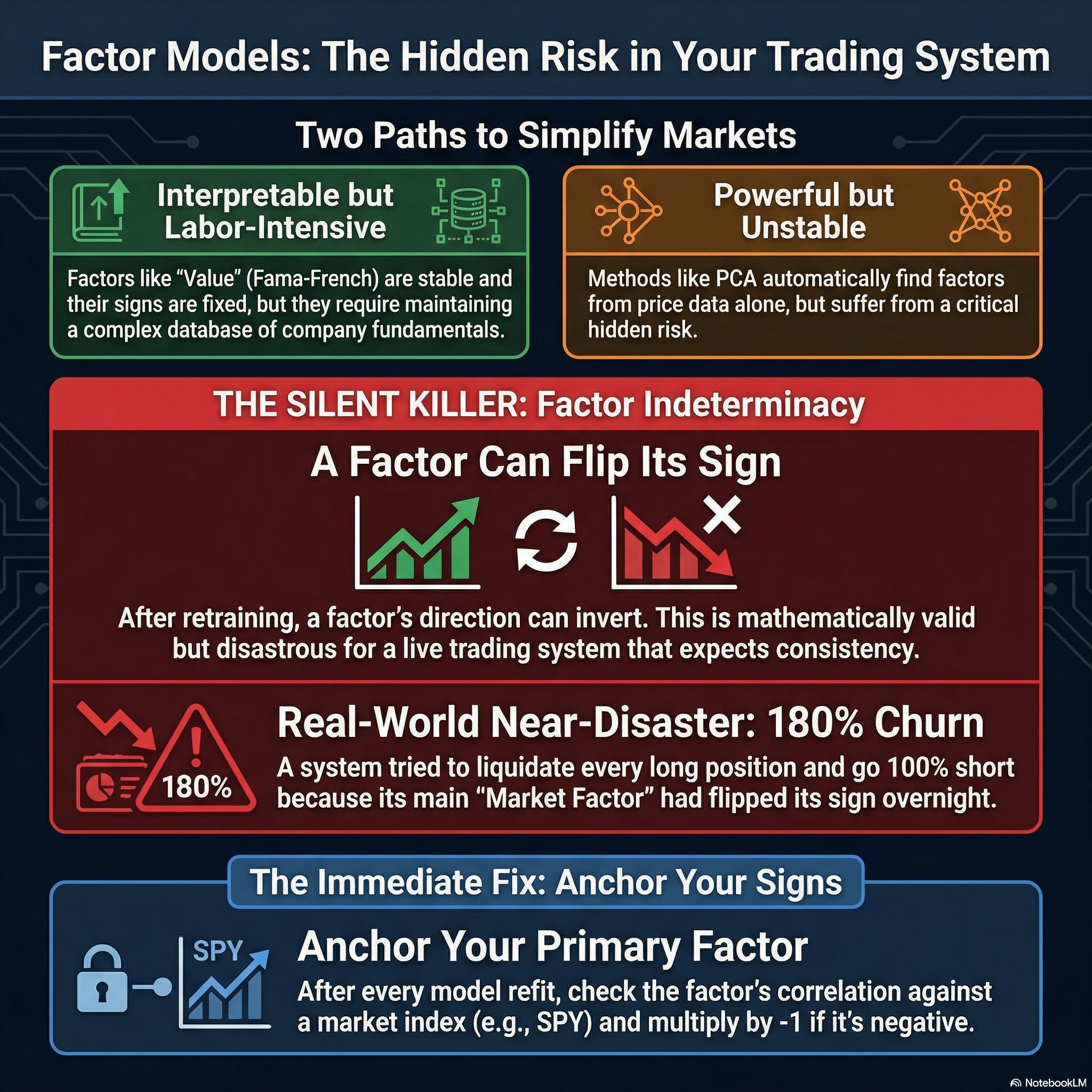
Last year, during a scheduled Sunday night model retraining, my system attempted to liquidate every long position and flip to 100% short. The predicted turnover alert showed 180% portfolio churn—roughly 5% in slippage and commissions for zero net change in actual exposure.
The root cause: a single eigenvector in my factor model changed sign.
If I hadn't built turnover constraints as a guardrail, the system would have executed the trades. For solo operators, this failure mode is particularly dangerous: it is not caught by code review, I don’t have a risk desk monitoring overnight, nor a team to catch edge cases. My system is limited to the high-level objective it is optimizing: in this case, this turned out to be mis-aligned.
This post covers factor models for dimensionality reduction — why design choices for these matter more than most tutorials admit, and a deep dive into the indeterminacy problem. If you're building systems that must estimate covariance, construct portfolios, or generate signals across thousands of instruments, this decomposition is foundational.
Factor Models
A portfolio of thousands of stocks implies storing and processing thousands of return series. But the effective dimensionality is far lower. Stocks tend to move together — driven by market sentiment, sector rotation, shared economics and macro forces.
Factor models reduce the dimensionality of a dataset down to a small number of factors affecting many instruments, plus idiosyncratic noise specific to each. The linear K-factor model:
where:
R_{i,t} = return of instrument i at time t
α_i = instrument-specific intercept
λ_ik = exposure (loading) of instrument i to factor k
f_{k,t} = return of factor k at time t
ε_{i,t} = idiosyncratic return specific to i (the part factor models can’t explain: a residual)
A small number of factors (e.g., K=5) can explain much of the variation in returns across thousands of instruments. If estimating covariances, instead of having to estimate O(N^2) parameters for a covariance matrix over N instruments, we only need to estimate O(KN) — orders of magnitude fewer.
The question: how do you estimate factors and loadings? And critically for autonomous systems: what fails silently when you choose wrong?
Economic vs Statistical Factors
Finance practitioners use the Capital Asset Pricing Model (CAPM) and Fama-French (FF) factors. ML engineers use Principal Components Analysis (PCA) and Autoencoders. For asset pricing, these are all equivalent (under mild assumptions of linearity).
Economic Factor Models: Stable but Generic
Economic factor models fix the basis ex-ante. Such factors are computed from economic theory and historical anomalies. These factors are designed to be interpretable and stable.
The CAPM is the most aggressive compression: a single factor explains expected excess returns as
where:
E[R_i] is the expected return on instrument i.
E[R_m] is the expected market return (e.g., the S&P 500).
R_f is the risk-free rate (e.g., the 2-year Treasury yield).
β_i is the market beta (systematic risk).
The entire cross-section of expected returns collapses to a single number per instrument i: the market beta. We estimate it by regressing an instrument’s excess returns on the market’s excess returns.
Fama-French (FF) Factors
Fama and French observed that CAPM leaves systematic patterns unexplained. The 3-factor model adds size (SMB: Small Minus Big) and value (HML: High Minus Low book-to-market). The 5-factor model extends this with profitability (RMW) and investment (CMA). All told, the Fama-French 5-factor model uses:
Market (MKT): CAPM beta
Size (SMB): Small Minus Big market cap
Value (HML): High Minus Low book-to-market
Profitability (RMW): Robust Minus Weak
Investment (CMA): Conservative Minus Aggressive
Factor returns are constructed from sorted portfolios—details available from Ken French’s data library.
The Trdeoffs with Economic Factors
Advantages:
Interpretable (you know what “value exposure” means)
Stable in sign and semantics (more on this below)
Predictable out-of-sample behavior
Limitations:
Generic dimensions are possibly not optimal for your specific universe of instruments
Requires point-in-time fundamentals (P/E, Market Cap)
Nonlinear relationships ignored
Data engineering tax: cleaning and maintaining corporate actions/metadata
For a solo operator, this last point matters. Maintaining an institutional-grade fundamental database is non-trivial manual labor in a system that is supposed to be autonomous.
Statistical Factor Models
Statistical factor models estimate factors and loadings jointly from data, by minimizing reconstruction error between observed returns and model estimates:
Principal Components Analysis (PCA) finds the K-dimensional subspace maximizing preserved variance. In PCA, we model returns using a linear K-factor model:
where \mu is the mean of N returns across time and \Lambda is a N x K loading matrix whose columns are the top K eigenvectors of the returns’ covariance matrix. The factors that minimize reconstruction error are:
No economic priors or fundamentals — just linear algebra and enough data to estimate parameters across thousands of stocks. Empirically, the first few PCA factors correlate strongly with Fama-French factors, as expected under factor equivalence. Despite equivalence, PCA has a property that will bite you in production: eigenvector signs are arbitrary.
Autoencoders
PCA finds the best linear compression of your returns. But what if factor loadings depend on regime, or factors interact multiplicatively? Autoencoders introduce nonlinearity via neural networks: the encoder maps from returns to a lower-dimensional variables z_t:
while the decoder maps this back to a reconstructed returns vector:
Here is some PyTorch for a simple 1-layer autoencoder:
import torch.nn as nn

class LinearDecoderAutoencoder(nn.Module):
    """
    Nonlinear encoder, linear decoder.
    Linear decoder preserves APT compatibility.
    """
    def __init__(self, n_assets: int, n_factors: int, hidden: int = 64):
        super().__init__()
        self.encoder = nn.Sequential(
            nn.Linear(n_assets, hidden),
            nn.ReLU(),
            nn.Linear(hidden, n_factors),
        )
        self.decoder = nn.Linear(n_factors, n_assets, bias=False)

    def forward(self, x):
        z = self.encoder(x)
        return self.decoder(z), z

    @property
    def loadings(self):
        return self.decoder.weight  # (N, K)
With linear activations and MSE loss, an autoencoder recovers PCA exactly. Nonlinear encoders with linear decoders can capture curved manifolds while preserving the factor structure. But autoencoders also inherit PCA's indeterminacy problem.
The Silent Killer: Factor Indeterminacy in Production
Now back to my Sunday night almost-disaster.
My trading system at the time was modular. The factor model saved updated loadings after retraining. The downstream portfolio optimizer (which was not re-trained) pulled these loadings prior to market open.
The first principal component — the “Market Factor” — had flipped its sign. This is mathematically valid: variance explained remains identical whether the eigenvector points “up” or “down.”
The optimizer interpreted the reversed factor direction as requiring a complete portfolio reorientation. Essentially the optimizer thought that everything previously positively exposed to markets is now negatively exposed — flip the entire book.
180% turnover, 5% in transaction costs and zero change in actual risk exposure.
This issue was caught because I’d built a turnover constraint into the optimizer. The predicted turnover alert fired. I killed trading before market open and spent the next week debugging. If I hadn't built that guardrail, the system would have executed the trades.
For solo operators, this is dangerous. You don’t have a team to catch edge cases during code review. You don’t have a risk desk monitoring overnight refits. Your system’s understanding of itself is your risk management.
Three Fixes for Factor Indeterminacy
Fix 1: Sign Anchoring (Quick Patch)
After every fit, check the correlation of the first latent factor against a broad market ETF (like SPY). If negative, multiply the entire factor and its corresponding loadings by -1.
This works, but it’s a brittle patch on a system that’s fundamentally blind to its global objective. You’re spending time writing guardrails because your modules operate under mutually incompatible assumptions.
Fix 2: Use Economic Factors (Trade Indeterminacy for Data Engineering)
Eschew the voodoo of statistical factor models and stick to economic ones, as these don’t have the indeterminacy issue. Since economic factors (like Fama-French) are hard-coded (they’re constructed by human-defined rules like “Small Minus Big”, or SMB) their signs are immutable. The “direction” is baked into the SQL query, not learned by an optimizer.
But this replaces a math problem with a data engineering tax. You must ingest, clean, and align point-in-time fundamental data for every instrument — at all times. You trade indeterminacy risk for the manual labor of maintaining an institutional-grade fundamental database.
Fix 3: End-to-End Differentiable Systems (The Clean Solution)
Design a system where the sign of factors is enforced by P&L itself: what we ultimately care about. If any factor flips its sign, the system should treat this as a catastrophic loss and self-correct as part of learning.
This requires moving from modular pipelines (factor model → optimizer) to end-to-end differentiable architectures where portfolio allocation decisions backpropagate through the entire stack. The factor model’s latent representations are optimized directly for trading performance, not reconstruction error.
Implementation requires careful handling of market execution, and designing loss functions that balance returns, risk, and turnover. Expect a post on this architecture in the future.
Key Takeaways
Factor model choice is an infrastructure decision, not just a statistical one:
Economic factors = high maintenance, low risk
Statistical factors = low maintenance, subtle risks
For solo operators: pick your poison based on what you can automate
Modular systems require explicit compatibility guarantees:
My factor model and optimizer operated under mutually incompatible assumptions
Module boundaries hide failure modes
More components = more edge cases you won’t catch alone
Turnover constraints are non-negotiable:
Your monitoring system must scream at unusual predicted turnover
Set thresholds based on historical patterns
This guardrail saved me 5% in unnecessary transaction costs
As a solo operator, your alerts are your risk desk
Statistical elegance ≠ production robustness:
PCA is mathematically elegant, but sign indeterminacy is a footnote in academic papers. In production with modular systems, it’s a portfolio-liquidating bug
The autonomous trading tax:
Every “low maintenance” choice has hidden failure modes
You discover these alone, at 3 AM, during market hours
Document your fixes—future you will face similar decisions
For solo operators: you don’t have the luxury of specialization. You must understand the entire stack, from linear algebra to production. This is necessary because failures compound across module boundaries and it’s on your system to catch them.
The eigenvector sign flip was mathematically valid. The portfolio liquidation would have been operationally catastrophic. That gap is where solo algorithmic traders earn their edge, or blow up their accounts.